-2.jpg?width=240&height=83&name=Menu-Banner%20(5)-2.jpg)
.jpg?width=240&height=83&name=Menu-Banner%20(8).jpg)


Overview
In the movie “The Core” [spoiler alert!] there is a great example (completely made-up, of course) of a theoretical element called (with tongue in cheek) Unobtanium. It has the unique property that it becomes stronger (gains structural integrity) as it is exposed to increasing levels of heat and pressure. So, it turns out to be the ideal material to build the fantastic ship they use to journey to the center of the Earth. Unobtanium strikes me as an idealized example of an antifragile physical material: A scene from “The Core” illustrating the physical magic of Unobtainium.
YouTube. A scene from “The Core” illustrating the physical magic of Unobtainium.
Most materials, when exposed to sufficient heat, would decompose, melt, or sublimate (undergo phase change) into the next stable higher energy state. For instance, when you boil water, it turns to steam. When you heat ice, it melts into water. When you hammer a physical material (say, a rock), it shatters into smaller pieces, and so on. In contrast, unobtanium becomes stronger and more rigid as it is taken deeper into the Earth’s core, where the temperatures and pressures are much higher than on the surface. The fact that it gains nonlinearly from the disorder in its environment means that it has antifragile characteristics. In the real world, certain fluids do exhibit convexity of response under stress – such fluids are called non-Newtonian, as they do not obey the classic Newtonian or linear response function in response to the addition of energy to the system. Well-known examples include silly-putty, quicksand, etc. – the more you stress them, the more they resist deformation.
YouTube. An explanation of non-Newtonian fluids.
Materials science is increasingly taking advantage of such nonlinear properties in the development of new materials that can withstand unusual conditions.
So, how does this apply to AI or machine learning?
Machine learning uses data (signal or information) to make predictions. The signal or information content of the data we have is the opposite of noise. If we think of the signal as having a sort of layered structure, then noise is the aspect of the signal that has no structure – it is random. From this randomness, no further information can be extracted. This is the limit of what a machine learning algorithm can learn from data. If we look at the performance of machine learning systems, we will observe they often have one or more optima. More often than not, we are looking at a performance curve that has an optimal level of noise corresponding to the error term in the formulation of a neural network.
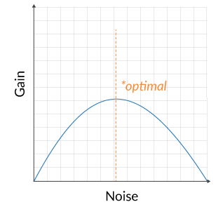
For stationary systems in which the machine learning process is looking to capture an unknown but unchanging phenomenon, the performance characteristics of the learning system would look something like this in response to noisy data.
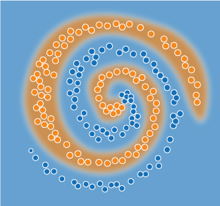
In the above diagram, there is an optimal level of noise in the data for which we see an improvement in model performance (“gain”), but beyond which the model performance decays rapidly. In fact, practitioners will often exploit this point to improve the learning process. For instance, I exploited this fact to get the following result for the open problem on one of the TensorFlow sample problems found online (the double spiral):
To be clear, the additive noise mixed into the data has no inherent structure. It is not an information-loaded stressor as described in the examples of cats and chess. That is a key point. The question is whether the stressor contains any new information or whether it is merely random noise that can be explained by a simple linear noise model. If the stressor is novel, it is certain to contain new information – for stationary systems, and this happens when we widen our sample (for instance). In other words, our first sample did not sufficiently capture the phenomenon we were interested in, and the second sample caught something new. However, for stationary systems, sampling eventually converges to the true distribution. For non-stationary systems, no matter how much you sample, you are unlikely to capture all the uncertainty/variability that is possible. It is in this latter situation where we can have a meaningful discussion about antifragility – because our interest in being antifragile is not with the assurance that we have captured “the process” – it is with the assurance that we don’t know what “the process” looks like, and we don’t need to know – all we need to know is that our process can adapt to whatever new things happen.
Notice how the spiral model generalizes the underlying spiral pattern well without overfitting the data. The separation between the boundary layers is smooth, not choppy. The spiral edges are not jagged, they are gently curving. Studying this double spiral problem with a critical eye can give you great insight into what a good model looks like and feels like. It can also help you gain a subtle appreciation for how parameters and hyperparameters affect training and learning.
In a very general sense, machine learning benefits from exposure to novel data, which helps improve its performance. However, we need to partition this into two different groups of machine learning problems to see precisely where the term antifragility truly applies. I find it trivial to call classical stationary machine learning problems as being “antifragile” – it is kind of cheating actually to claim this because we know apriori that such problems do not have an endless parade of novelstressors.
Antifragility only applies to non-stationary contexts
When the underlying process is stationary (which is true for the vast majority of classical ML applications), this “learning” happens up to a point (in theory, the limit of the total signal or information contained in the data), and then further optimization tends to worsen the outcome as this signal gets diluted. This cannot constitute antifragility simply because the underlying system itself is unlikely to produce any major unexpected shocks or stressors, as it follows the assumptions of a simple GLM (generalized linear model) process. We know that for the alternate case where the underlying process undergoes a radical change, the simple machine learning model built for the stationary case may not be able to adapt. The point of antifragility is that we don’t know what will happen next! So, if our model only works under the assumption of stationarity, linearity, or some other bias, we are not building for antifragility, even though we are using a machine learning model. When the underlying system is unlikely to produce any novel stressors, a simple classical linear machine learning model is likely to converge on a solution that won’t change for very long periods of time – and that linear bias may be useful to claim robustness, but it is contrary to our goal of achieving antifragility.
In the real world, long-term processes (e.g., major market trends or “fads”) can take months or years to develop, play out, and die out. These can be modeled as approximately linear in any subset of the time course of the evolution of these trends – so, classical machine learning models adapt to these changes by relying on a physical process of refreshing the model parameters (retraining) after some period of use. In contrast, the more modern “dynamic” models are useful when the same underlying trends and processes change fast. In those situations, we have to determine whether the process is stationary or non-stationary. Again, most problems that excite us about deploying deep learning still have many stationary characteristics. Learning what cats look like (for all intents and purposes) is (kind of) globally stationary, even if it is locally non-stationary. Getting a complete representation of cats is largely a sampling problem. But, now let me argue the opposite, here’s why it is not globally stationary: We are ignoring the fact that cats exist in a larger context where they are forced to evolve by natural selection – so they serve as a source of novelty because genetic mutations and natural selection cause the “cat generating process” to produce new kinds of cats all the time. The underlying ML algorithm, if it is based on deep learning principles (layered network architecture, distributed feature representation, multi-scale representations, etc.), will likely keep up and even evolve its definition of a “cat” no matter how weird the cats start to look over time. Such a system could be called truly “antifragile”. Antifragility seems only meaningful for non-stationary systems in which novel stressors keep coming, in an endless parade of novelty. The tendency to antifragility is more strongly observed in machine learning systems where the underlying processes being learned are complex, non-stationary, and have an open-ended number of possible solutions. This is evident in games such as chess, where the rules are known apriori, and the combinations of gameplay are virtually infinite. When we employ machine learning (e.g., adversarial deep learning) to have one machine play against another machine, the two machines learn by competing with each other – essentially stressing each other through an unending stream of novel tactics (moves). As they stress each other (in order to kill each other), they both gain from each encounter over time – allowing the system to evolve new strategies or tactics that no human had ever considered before.
Conclusion
By adding selective noise to the training data, we can improve model robustness and generalization as well as achieve greater stability. This leads to models that are less likely to be “over-fit” and more likely to generalize to the underlying true behavior of the process they are trying to capture. Now, people often confuse robustness with anti-fragility, but they are not the same thing. Robustness means that a model is less likely to be seriously negatively impacted by shocks or unexpected variances in the inputs. Robustness does not imply that a model necessarily gains from those shocks, it merely assures us that we are less likely to be over-fit to the data. An analogy that I like is that of a well-tailored suit that loosely fits your body: You don’t want a suit that stops fitting you if you gain a pound or two. You also don’t want a suit that is too big